Today we’re talking about bandits. Bandit problems, not dissimilar from Markov chains, are one of those simple models that apply to a wide variety of problems. Indeed, many results of “sequential decision making” stem from the study of bandit problems. Plus the name is cool, so that should provide some motivation for wanting to study them. The name bandit originates from the term one-armed bandit, which was used to describe slot machines.

In their survey on bandits, Bubeck and Cesa-Bianchi define a multi-armed bandit problem as “a sequential allocation problem defined by a set of actions.” The allocation problem is similar to a (repeated) game: at each point in time, the player chooses an action i.e., an arm, and receives a reward.

The player’s goal is to maximize her cumulative reward, which naturally leads to an exploitation vs. exploration problem. The player needs to simultaneously exploit arms known to yield high rewards and explore other arms in the hopes of finding other high-yield rewards.

In bandit problems, we assess a player’s performance by her regret, which compares her performance to (something like) the best-possible performance. After the first $n$ rounds of the game, the player’s regret is

$$R_n = \max_{i=1,\dots,K} \sum_{i=1}^n X_{i,t} - \sum_{i=1}^n X_{I_t,t},$$

where $K$ is the number of bandit arms, $X_{i,t}$ is the reward of arm $i$ at time $t$, and $I_t$ is the player’s (possibly randomly) chosen arm.

Stochastic bandit problems

In this post, we’re going to focus on stochastic bandit problems as opposed to adversarially bandit problems. Here’s the set-up.

• There are $\{1,\dots,K\}$ arms.
• Each arm $i$ corresponds to an unknown probability distribution $p_i$.
• At each time $t$, the player selects an arm $I_t$ (independently of previous choices) and receives a reward $X_{I_t,t} \sim p_{I_t}$.

We’ll denote the mean of distribution $i$ with $\mu_i$ and define

$$\mu^\star = \max_{i=1,\dots,K} \mu_i \quad \textsf{and} \quad i^\star = \argmax_{i=1,\dots,K} \mu_i$$

as optimal parameters. Instead of using the regret to assess our player’s performance, we’ll use the pseudo-regret, which is defined as

$$\begin{align*} \bar{R}_n &= \max_{i=1,\dots,K} \E \left[ \sum_{i=1}^n X_{i,t} - \sum_{i=1}^n X_{I_t,t} \right] \\ &= n \mu^\star - \E \sum_{t=1}^n \mu_{I_t}. \end{align*}$$

We know that $\bar{R}_n \le \E R_n$ because of Jensen’s inequality for convex functions. For our purposes, a more informative form of the pseudo-regret is

$$\bar{R}_n = \sum_{i=1}^K \Delta_i \E T_i(n),$$

where $\Delta_i = \mu^\star - \mu_i$ is the suboptimality of arm $i$ and the random variable $T_i(n) = \sum_{i=1}^n \ind{}\{I_t = i\}$ is the number of times arm $i$ is selected in the first $n$ rounds.

This alternative expression for the pseudo-regret sums over arms rather than rounds. To see how we switched from arms to rounds, play around with random variables $T_i(n)$.

Upper confidence bounds

One approach for simultaneously performing exploration and exploitation is to use upper confidence bound (UCB) strategies. UCB strategies produce upper bounds (based on a confidence level) on the current estimate for each arm’s mean reward. The player selects the arm that is the best using the UCB-modified estimate.

In the spirit of brevity, we’re going to gloss over a few important details (e.g., Legendre–Fenchel duals and Hoeffding’s lemma) but here’s the gist of the UCB set-up.

• Define $\widehat{\mu}_{i,n} = \frac{1}{n} \sum_{j=1}^n X_{i,j}$ as the sample mean of arm $i$ after being played $n$ times.
• For a convex function $\psi$ with convex conjugate $\psi^*$ and parameter $\lambda > 0$, the cumulant generating function of $X$ is bounded by $\psi$:

$$\ln \E e^{\lambda(X - \E X)} \le \psi(\lambda) \quad \textsf{and} \quad \ln \E e^{\lambda(\E X - X)} \le \psi(\lambda).$$

• By Markov’s inequality and the Cramér–Chernoff technique

$$\prob \left( \mu_i - \widehat{\mu}_{i,n} \ge \varepsilon \right) \le e^{-n \psi^*(\varepsilon)}.$$

• Markov’s inequality means that, with probability $1 - \delta$, we have an upper bound on the estimate of the $i$th arm:

$$\mu_i < \widehat{\mu}_{i,n} + (\psi^*)^{-1} \left(\frac{1}{n} \ln \frac{1}{\delta} \right).$$

The UCB strategy is (very) simple; at each time $t$, select the arm $I_t$ by

$$I_t \in \argmax_{i=1,\dots,K} \left\{ \widehat{\mu}_{i,T_i(t-1)} + (\psi^*)^{-1} \left( \frac{\alpha \ln t}{T_i(t-1)} \right) \right\}.$$

The tradeoff. Let’s pick apart this term and see how it encourages exploration and exploitation. We’re going to use $\psi(x) = x^2/8$ with convex conjugate $\psi^*(z) = 2z^2$, so that $(\psi^*)^{-1}(z) = (x/2)^{1/2}$.

When arm $i$ has not been played many times before time $t$, i.e., when $T_i(t-1)$ is small numerator of $\frac{\alpha \ln t}{T_i(t-1)}$ dominates and the UCB-adjusted estimate of arm $i$ is likely to relatively high, which encourages arm $i$ to be chosen. In other words, it encourages exploration.

As arm $i$ is chosen more, $T_i(t-1)$ increases and the estimate $\widehat{\mu}_{i,T_i(t-1)}$ improves. If arm $i$ is the optimal arm, then the $\widehat{\mu}_{i,T_i(t-1)}$ term dominates the estimates for other arms and the UCB-adjustment further encourages selection of this arm. This means that the algorithm exploits high-yielding arms.

Upper bound on pseudo-regret. If our player follows the UCB scheme specified above, then for $\alpha > 2$ her pseudo-regret is upperbounded as

$$\bar{R}_n \le \sum_{i: \Delta_i > 0} \left( \frac{\alpha \Delta_i}{\psi^*(\Delta_i / 2)} \ln n + \frac{\alpha}{\alpha - 2} \right).$$

We’re going to prove the bound in the next post.

Bandit simulations

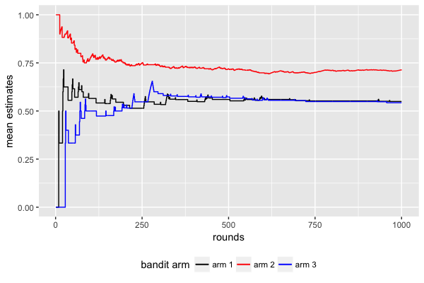
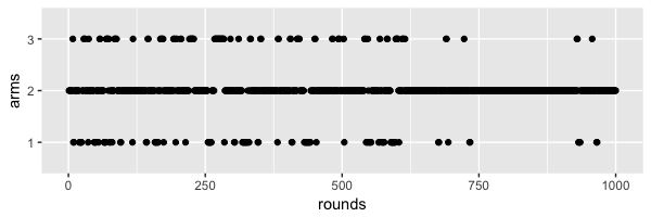
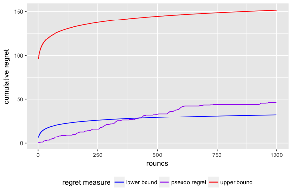
Here’s an R script which uses the upper confidence bound algorithm. For the plots below, there are $K = 3$ arms and $n = 1000$ rounds. The reward distributions are Bernoulli’s and the mean parameters the three arms are 0.46, 0.72, and 0.55.

The first plot shows the evolution of each mean estimate as different rounds are played.

The next plot illustrates the exploration vs. exploitation trade-off. Even though arm 2 yields the highest rewards, the algorithm occasionally plays arms 1 and 3 in later rounds.

The final plot shows the player’s cumulative regret compared to the UCB-implied upper bound on the regret; the lower bound is distribution-dependent and asymptotic, which is why it exceeds the pseudo-regret until round 400ish.

Next up

… a proof of the upper confidence bound regret rate!

References

This post is based on material from:

• Regret Analysis of Stochastic and Nonstochastic Multi-armed Bandit Problems by S. Bubeck and N. Cesa-Bianchi. A digital copy can be found here.
• Prediction, Learning, and Games (a.k.a. “Perdition, Burning, and Flames”) by N. Cesa-Bianchi and G. Lugosi. Find a description of the book and its table of contents here.

I would also recommend checking out Sébastien Bubeck’s blog “I’m a bandit” and, in particular, his bandit tutorials: part 1 and part 2. Also check out his new YouTube channel: https://www.youtube.com/user/sebastienbubeck/videos.